ClickHouse는 쿼리를 매우 빠르게 처리하지만, 쿼리 실행 과정은 그리 단순하지 않습니다. SELECT 쿼리가 어떻게 실행되는지 이해해 보겠습니다. 이를 설명하기 위해 ClickHouse의 한 테이블에 데이터를 몇 개 추가해 보겠습니다:
CREATE TABLE session_events(
   clientId UUID,
   sessionId UUID,
   pageId UUID,
   timestamp DateTime,
   type String
) ORDER BY (timestamp);

INSERT INTO session_events SELECT * FROM generateRandom('clientId UUID,
   sessionId UUID,
   pageId UUID,
   timestamp DateTime,
   type Enum(\'type1\', \'type2\')', 1, 10, 2) LIMIT 1000;
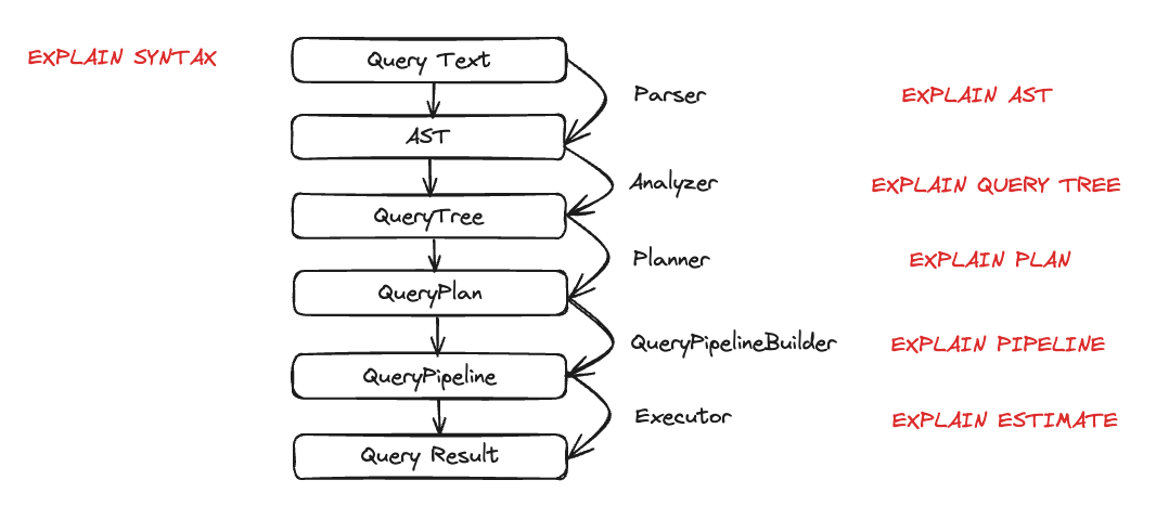
이제 ClickHouse에 어느 정도 데이터가 적재되었으므로, 쿼리를 실행하고 그 실행 방식을 이해해 보겠습니다. 쿼리 실행은 여러 단계로 분해됩니다. 쿼리 실행의 각 단계는 해당하는 EXPLAIN 쿼리를 사용하여 분석하고 문제를 진단 및 해결할 수 있습니다. 이러한 단계는 아래 차트에 요약되어 있습니다:
이제 쿼리 실행 중에 각 구성 요소가 실제로 어떻게 동작하는지 살펴보겠습니다. 몇 가지 쿼리를 실행한 뒤 EXPLAIN 구문을 사용해 이를 분석해 보겠습니다.
파서(Parser)
파서의 목적은 쿼리 텍스트를 AST(Abstract Syntax Tree)로 변환하는 것입니다. 이 단계는 EXPLAIN AST 명령으로 시각화할 수 있습니다.
EXPLAIN AST SELECT min(timestamp), max(timestamp) FROM session_events;

┌─explain────────────────────────────────────────────┐
│ SelectWithUnionQuery (children 1)                  │
│  ExpressionList (children 1)                       │
│   SelectQuery (children 2)                         │
│    ExpressionList (children 2)                     │
│     Function min (alias minimum_date) (children 1) │
│      ExpressionList (children 1)                   │
│       Identifier timestamp                         │
│     Function max (alias maximum_date) (children 1) │
│      ExpressionList (children 1)                   │
│       Identifier timestamp                         │
│    TablesInSelectQuery (children 1)                │
│     TablesInSelectQueryElement (children 1)        │
│      TableExpression (children 1)                  │
│       TableIdentifier session_events               │
└────────────────────────────────────────────────────┘
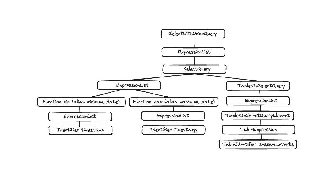
출력은 아래와 같이 시각화할 수 있는 추상 구문 트리(Abstract Syntax Tree)입니다.
각 노드는 자식 노드를 가지며, 전체 트리는 쿼리의 전체 구조를 나타냅니다. 이는 쿼리를 처리하는 데 도움이 되는 논리적 구조입니다. 엔드유저 관점에서는 (쿼리 실행에 관심이 있는 경우가 아니라면) 크게 유용하지 않으며, 이 도구는 주로 개발자가 사용하는 도구입니다.
Analyzer
현재 ClickHouse에는 Analyzer를 위한 두 가지 아키텍처가 있습니다. enable_analyzer=0 을 설정하면 기존 아키텍처를 사용할 수 있습니다. 새로운 아키텍처는 기본적으로 활성화되어 있습니다. 새로운 analyzer가 일반적으로 사용 가능해지면 기존 아키텍처는 사용 중단(deprecated)될 예정이므로, 여기서는 새로운 아키텍처만 설명합니다.
참고
새로운 아키텍처는 ClickHouse의 성능을 개선하기 위한 더 나은 프레임워크를 제공합니다. 그러나 쿼리 처리 단계의 근본적인 구성 요소이기 때문에 일부 쿼리에 부정적인 영향을 줄 수도 있으며, 알려진 비호환성이 존재합니다. 쿼리 또는 USER 수준에서 enable_analyzer SETTING을 변경하여 기존 analyzer로 되돌릴 수 있습니다.
Analyzer는 쿼리 실행에서 중요한 단계입니다. Analyzer는 AST를 받아 쿼리 트리로 변환합니다. 쿼리 트리가 AST보다 가지는 주요 이점은, 예를 들어 스토리지와 같이 많은 구성 요소들이 미리 해결(resolved)된다는 점입니다. 어떤 테이블에서 읽을지 알 수 있고, 별칭(alias)도 해결되며, 트리는 사용되는 서로 다른 데이터 타입도 알고 있습니다. 이러한 모든 이점을 바탕으로 analyzer는 최적화를 적용할 수 있습니다. 이러한 최적화는 「패스(pass)」를 통해 동작합니다. 각 패스는 서로 다른 최적화를 탐색합니다. 모든 패스는 여기에서 확인할 수 있으며, 이전에 사용했던 쿼리를 가지고 실제로 어떻게 동작하는지 살펴보겠습니다:
EXPLAIN QUERY TREE passes=0 SELECT min(timestamp) AS minimum_date, max(timestamp) AS maximum_date FROM session_events SETTINGS allow_experimental_analyzer=1;

┌─explain────────────────────────────────────────────────────────────────────────────────┐
│ QUERY id: 0                                                                            │
│   PROJECTION                                                                           │
│     LIST id: 1, nodes: 2                                                               │
│       FUNCTION id: 2, alias: minimum_date, function_name: min, function_type: ordinary │
│         ARGUMENTS                                                                      │
│           LIST id: 3, nodes: 1                                                         │
│             IDENTIFIER id: 4, identifier: timestamp                                    │
│       FUNCTION id: 5, alias: maximum_date, function_name: max, function_type: ordinary │
│         ARGUMENTS                                                                      │
│           LIST id: 6, nodes: 1                                                         │
│             IDENTIFIER id: 7, identifier: timestamp                                    │
│   JOIN TREE                                                                            │
│     IDENTIFIER id: 8, identifier: session_events                                       │
│   SETTINGS allow_experimental_analyzer=1                                               │
└────────────────────────────────────────────────────────────────────────────────────────┘
EXPLAIN QUERY TREE passes=20 SELECT min(timestamp) AS minimum_date, max(timestamp) AS maximum_date FROM session_events SETTINGS allow_experimental_analyzer=1;

┌─explain───────────────────────────────────────────────────────────────────────────────────┐
│ QUERY id: 0                                                                               │
│   PROJECTION COLUMNS                                                                      │
│     minimum_date DateTime                                                                 │
│     maximum_date DateTime                                                                 │
│   PROJECTION                                                                              │
│     LIST id: 1, nodes: 2                                                                  │
│       FUNCTION id: 2, function_name: min, function_type: aggregate, result_type: DateTime │
│         ARGUMENTS                                                                         │
│           LIST id: 3, nodes: 1                                                            │
│             COLUMN id: 4, column_name: timestamp, result_type: DateTime, source_id: 5     │
│       FUNCTION id: 6, function_name: max, function_type: aggregate, result_type: DateTime │
│         ARGUMENTS                                                                         │
│           LIST id: 7, nodes: 1                                                            │
│             COLUMN id: 4, column_name: timestamp, result_type: DateTime, source_id: 5     │
│   JOIN TREE                                                                               │
│     TABLE id: 5, alias: __table1, table_name: default.session_events                      │
│   SETTINGS allow_experimental_analyzer=1                                                  │
└───────────────────────────────────────────────────────────────────────────────────────────┘
두 번의 실행 결과를 비교하면 별칭(alias)과 프로젝션이 어떻게 해석되는지 확인할 수 있습니다.
Planner
Planner는 쿼리 트리를 입력으로 받아 쿼리 플랜을 생성합니다. 쿼리 트리는 특정 쿼리로 무엇을 수행하려는지를 나타내고, 쿼리 플랜은 이를 어떻게 수행할지를 나타냅니다. 추가적인 최적화는 쿼리 플랜 단계에서 수행됩니다. EXPLAIN PLAN 또는 EXPLAIN을 사용하여 쿼리 플랜을 확인할 수 있으며, EXPLAIN은 내부적으로 EXPLAIN PLAN을 실행합니다.
EXPLAIN PLAN WITH
   (
       SELECT count(*)
       FROM session_events
   ) AS total_rows
SELECT type, min(timestamp) AS minimum_date, max(timestamp) AS maximum_date, count(*) /total_rows * 100 AS percentage FROM session_events GROUP BY type

┌─explain──────────────────────────────────────────┐
│ Expression ((Projection + Before ORDER BY))      │
│   Aggregating                                    │
│     Expression (Before GROUP BY)                 │
│       ReadFromMergeTree (default.session_events) │
└──────────────────────────────────────────────────┘
이 정보도 어느 정도 도움이 되지만, 더 많은 정보를 얻을 수 있습니다. 예를 들어, 프로젝션을 생성해야 하는 대상 컬럼의 이름을 알고 싶을 수 있습니다. 이 경우 쿼리에 헤더를 추가하면 됩니다:
EXPLAIN header = 1
WITH (
       SELECT count(*)
       FROM session_events
   ) AS total_rows
SELECT
   type,
   min(timestamp) AS minimum_date,
   max(timestamp) AS maximum_date,
   (count(*) / total_rows) * 100 AS percentage
FROM session_events
GROUP BY type

┌─explain──────────────────────────────────────────┐
│ Expression ((Projection + Before ORDER BY))      │
│ Header: type String                              │
│         minimum_date DateTime                    │
│         maximum_date DateTime                    │
│         percentage Nullable(Float64)             │
│   Aggregating                                    │
│   Header: type String                            │
│           min(timestamp) DateTime                │
│           max(timestamp) DateTime                │
│           count() UInt64                         │
│     Expression (Before GROUP BY)                 │
│     Header: timestamp DateTime                   │
│             type String                          │
│       ReadFromMergeTree (default.session_events) │
│       Header: timestamp DateTime                 │
│               type String                        │
└──────────────────────────────────────────────────┘
이제 마지막 PROJECTION에서 생성해야 할 컬럼 이름인 minimum_date, maximum_date, percentage를 알게 되었지만, 실행해야 하는 모든 동작의 세부 내역도 확인하고 싶을 수 있습니다. 이때는 actions=1로 설정하면 됩니다.
EXPLAIN actions = 1
WITH (
       SELECT count(*)
       FROM session_events
   ) AS total_rows
SELECT
   type,
   min(timestamp) AS minimum_date,
   max(timestamp) AS maximum_date,
   (count(*) / total_rows) * 100 AS percentage
FROM session_events
GROUP BY type

┌─explain────────────────────────────────────────────────────────────────────────────────────────────────────────────────────────────────────┐
│ Expression ((Projection + Before ORDER BY))                                                                                                │
│ Actions: INPUT :: 0 -> type String : 0                                                                                                     │
│          INPUT : 1 -> min(timestamp) DateTime : 1                                                                                          │
│          INPUT : 2 -> max(timestamp) DateTime : 2                                                                                          │
│          INPUT : 3 -> count() UInt64 : 3                                                                                                   │
│          COLUMN Const(Nullable(UInt64)) -> total_rows Nullable(UInt64) : 4                                                                 │
│          COLUMN Const(UInt8) -> 100 UInt8 : 5                                                                                              │
│          ALIAS min(timestamp) :: 1 -> minimum_date DateTime : 6                                                                            │
│          ALIAS max(timestamp) :: 2 -> maximum_date DateTime : 1                                                                            │
│          FUNCTION divide(count() :: 3, total_rows :: 4) -> divide(count(), total_rows) Nullable(Float64) : 2                               │
│          FUNCTION multiply(divide(count(), total_rows) :: 2, 100 :: 5) -> multiply(divide(count(), total_rows), 100) Nullable(Float64) : 4 │
│          ALIAS multiply(divide(count(), total_rows), 100) :: 4 -> percentage Nullable(Float64) : 5                                         │
│ Positions: 0 6 1 5                                                                                                                         │
│   Aggregating                                                                                                                              │
│   Keys: type                                                                                                                               │
│   Aggregates:                                                                                                                              │
│       min(timestamp)                                                                                                                       │
│         Function: min(DateTime) → DateTime                                                                                                 │
│         Arguments: timestamp                                                                                                               │
│       max(timestamp)                                                                                                                       │
│         Function: max(DateTime) → DateTime                                                                                                 │
│         Arguments: timestamp                                                                                                               │
│       count()                                                                                                                              │
│         Function: count() → UInt64                                                                                                         │
│         Arguments: none                                                                                                                    │
│   Skip merging: 0                                                                                                                          │
│     Expression (Before GROUP BY)                                                                                                           │
│     Actions: INPUT :: 0 -> timestamp DateTime : 0                                                                                          │
│              INPUT :: 1 -> type String : 1                                                                                                 │
│     Positions: 0 1                                                                                                                         │
│       ReadFromMergeTree (default.session_events)                                                                                           │
│       ReadType: Default                                                                                                                    │
│       Parts: 1                                                                                                                             │
│       Granules: 1                                                                                                                          │
└────────────────────────────────────────────────────────────────────────────────────────────────────────────────────────────────────────────┘
이제 사용 중인 모든 입력, 함수, 별칭, 데이터 유형을 확인할 수 있습니다. 플래너가 적용할 일부 최적화는 여기에서 확인할 수 있습니다.
쿼리 파이프라인
쿼리 파이프라인은 쿼리 플랜으로부터 생성됩니다. 쿼리 파이프라인은 쿼리 플랜과 매우 유사하지만 트리가 아니라 그래프라는 점이 다릅니다. 이는 ClickHouse가 쿼리를 어떻게 실행하고 어떤 리소스를 사용할 것인지 보여줍니다. 쿼리 파이프라인을 분석하면 입출력 측면에서 병목 지점이 어디인지 파악하는 데 매우 유용합니다. 이전에 사용한 쿼리를 다시 사용해 쿼리 파이프라인 실행을 살펴보겠습니다:
EXPLAIN PIPELINE
WITH (
       SELECT count(*)
       FROM session_events
   ) AS total_rows
SELECT
   type,
   min(timestamp) AS minimum_date,
   max(timestamp) AS maximum_date,
   (count(*) / total_rows) * 100 AS percentage
FROM session_events
GROUP BY type;

┌─explain────────────────────────────────────────────────────────────────────┐
│ (Expression)                                                               │
│ ExpressionTransform × 2                                                    │
│   (Aggregating)                                                            │
│   Resize 1 → 2                                                             │
│     AggregatingTransform                                                   │
│       (Expression)                                                         │
│       ExpressionTransform                                                  │
│         (ReadFromMergeTree)                                                │
│         MergeTreeSelect(pool: PrefetchedReadPool, algorithm: Thread) 0 → 1 │
└────────────────────────────────────────────────────────────────────────────┘
괄호 안에는 쿼리 계획 단계가, 그 옆에는 프로세서가 표시됩니다. 매우 유용한 정보이지만, 이것이 그래프 구조인 만큼 실제 그래프로 시각화할 수 있다면 더 좋습니다. graph 설정을 1로 지정하고 출력 형식을 TSV로 설정할 수 있습니다:
EXPLAIN PIPELINE graph=1 WITH
   (
       SELECT count(*)
       FROM session_events
   ) AS total_rows
SELECT type, min(timestamp) AS minimum_date, max(timestamp) AS maximum_date, count(*) /total_rows * 100 AS percentage FROM session_events GROUP BY type FORMAT TSV;
digraph
{
 rankdir="LR";
 { node [shape = rect]
   subgraph cluster_0 {
     label ="Expression";
     style=filled;
     color=lightgrey;
     node [style=filled,color=white];
     { rank = same;
       n5 [label="ExpressionTransform × 2"];
     }
   }
   subgraph cluster_1 {
     label ="Aggregating";
     style=filled;
     color=lightgrey;
     node [style=filled,color=white];
     { rank = same;
       n3 [label="AggregatingTransform"];
       n4 [label="Resize"];
     }
   }
   subgraph cluster_2 {
     label ="Expression";
     style=filled;
     color=lightgrey;
     node [style=filled,color=white];
     { rank = same;
       n2 [label="ExpressionTransform"];
     }
   }
   subgraph cluster_3 {
     label ="ReadFromMergeTree";
     style=filled;
     color=lightgrey;
     node [style=filled,color=white];
     { rank = same;
       n1 [label="MergeTreeSelect(pool: PrefetchedReadPool, algorithm: Thread)"];
     }
   }
 }
 n3 -> n4 [label=""];
 n4 -> n5 [label="× 2"];
 n2 -> n3 [label=""];
 n1 -> n2 [label=""];
}
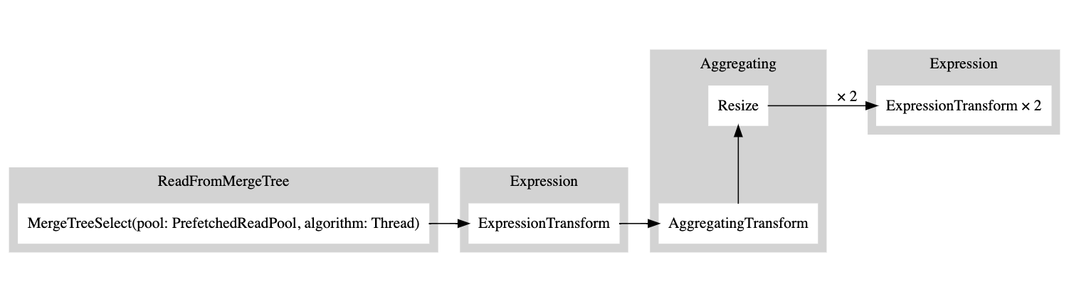
그런 다음 이 출력 결과를 복사하여 여기에 붙여넣으면 다음과 같은 그래프가 생성됩니다:
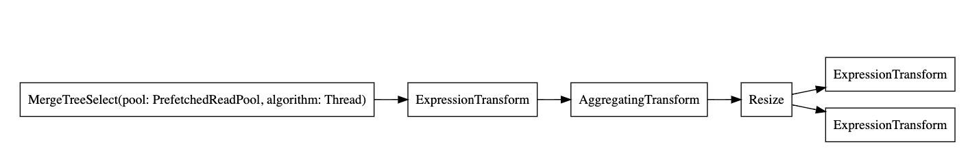
흰색 직사각형은 파이프라인 노드를, 회색 직사각형은 쿼리 플랜 단계(query plan steps)를 나타내며, x 뒤에 붙은 숫자는 사용 중인 입력/출력 개수를 의미합니다. 그래프를 축약된(compact) 형태로 보고 싶지 않다면, 언제든지 compact=0을 추가하면 됩니다:
EXPLAIN PIPELINE graph = 1, compact = 0
WITH (
       SELECT count(*)
       FROM session_events
   ) AS total_rows
SELECT
   type,
   min(timestamp) AS minimum_date,
   max(timestamp) AS maximum_date,
   (count(*) / total_rows) * 100 AS percentage
FROM session_events
GROUP BY type
FORMAT TSV
digraph
{
 rankdir="LR";
 { node [shape = rect]
   n0[label="MergeTreeSelect(pool: PrefetchedReadPool, algorithm: Thread)"];
   n1[label="ExpressionTransform"];
   n2[label="AggregatingTransform"];
   n3[label="Resize"];
   n4[label="ExpressionTransform"];
   n5[label="ExpressionTransform"];
 }
 n0 -> n1;
 n1 -> n2;
 n2 -> n3;
 n3 -> n4;
 n3 -> n5;
}
ClickHouse는 왜 여러 스레드를 사용해 테이블에서 읽지 않을까요? 테이블에 더 많은 데이터를 추가해 보겠습니다.
INSERT INTO session_events SELECT * FROM generateRandom('clientId UUID,
   sessionId UUID,
   pageId UUID,
   timestamp DateTime,
   type Enum(\'type1\', \'type2\')', 1, 10, 2) LIMIT 1000000;
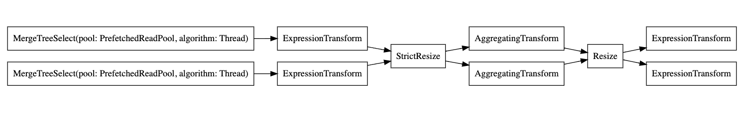
이제 다시 EXPLAIN 쿼리를 실행해 보겠습니다:
EXPLAIN PIPELINE graph = 1, compact = 0
WITH (
       SELECT count(*)
       FROM session_events
   ) AS total_rows
SELECT
   type,
   min(timestamp) AS minimum_date,
   max(timestamp) AS maximum_date,
   (count(*) / total_rows) * 100 AS percentage
FROM session_events
GROUP BY type
FORMAT TSV
digraph
{
  rankdir="LR";
  { node [shape = rect]
    n0[label="MergeTreeSelect(pool: PrefetchedReadPool, algorithm: Thread)"];
    n1[label="MergeTreeSelect(pool: PrefetchedReadPool, algorithm: Thread)"];
    n2[label="ExpressionTransform"];
    n3[label="ExpressionTransform"];
    n4[label="StrictResize"];
    n5[label="AggregatingTransform"];
    n6[label="AggregatingTransform"];
    n7[label="Resize"];
    n8[label="ExpressionTransform"];
    n9[label="ExpressionTransform"];
  }
  n0 -> n2;
  n1 -> n3;
  n2 -> n4;
  n3 -> n4;
  n4 -> n5;
  n4 -> n6;
  n5 -> n7;
  n6 -> n7;
  n7 -> n8;
  n7 -> n9;
}
그래서 executor는 데이터 양이 충분히 크지 않다고 판단해 연산을 병렬화하지 않았습니다. 더 많은 행을 추가하자 executor는 그래프에 표시된 것처럼 여러 스레드를 사용하도록 전환했습니다.
Executor
마지막으로 쿼리 실행의 최종 단계는 executor가 담당합니다. executor는 쿼리 파이프라인을 받아 이를 실행합니다. SELECT, INSERT, 또는 INSERT SELECT를 수행하는지에 따라 서로 다른 유형의 executor가 사용됩니다.